Classics in the History of Psychology

An internet resource developed by
Christopher D. Green
York University, Toronto, Ontario
ISSN 1492-3173

(Return to index)

STATISTICAL METHODS FOR RESEARCH WORKERS

43. We shall in this chapter give examples of the further applications of the method of the analysis of variance developed in the last chapter in connexion with the theory of intraclass correlations. It is impossible in a short space to give examples of all the different applications which may be made of this method; we shall therefore limit ourselves to those of the most immediate practical importance, paying especial attention to those cases where erroneous methods have been largely used, or where no alternative method of attack has hitherto been put forward.

There is no more pressing need in connexion with the examination of experimental results than to test whether a given body of data is or is not in agreement with any suggested hypothesis. The previous chapters have largely been concerned with such tests appropriate to hypotheses involving frequency of occurrence, such as the Mendelian hypothesis of [p. 212] segregating genes, or the hypothesis of linear arrangement in linkage groups, or the more general hypotheses of the independence or correlation of variates. More frequently, however, it is desired to test hypotheses involving, in statistical language, the form of regression lines. We may wish to test, for example, if the growth of an animal, plant or population follows an assigned law, if for example it increases with time in arithmetic or geometric progression, or according to the so-called "autocatalytic" law of increase; we may wish to test if with increasing applications of manure plant growth increases in accordance with the laws which have been put forward, or whether in fact the data in hand are inconsistent with such a supposition. Such questions arise not only in crucial tests of widely recognised laws, but in every case where a relation, however empirical, is believed to be descriptive of the data, and are of value not only in the final stage of establishing the laws of nature, but in the early stages of testing the efficiency of a technique. The methods we shall put forward for testing the Goodness of Fit of regression lines are aimed not only at simplifying the calculations by reducing them to a standard form, and so making accurate tests possible, but at so displaying the whole process that it may be apparent exactly what questions can be answered by such a statistical examination of the data.

If for each of a number of selected values of the independent variate x a number of observations of the dependent variate y is made, let the number of values of x available be a; then a is the number [p. 213] of arrays in our data. Designating any particular array by means of the suffix p, the number of observations in any array will be denoted by n_p, and the mean of their values by y[bar]_p; y[bar] being the general mean of all the values of y. Then whatever be the nature of the data, the purely algebraic identity

S(y-y[bar])² = S{n_p(y[bar]_p-y[bar])²} + SS(y-y[bar]_p)²

expresses the fact that the sum of the squares of the deviations of all the values of y from their general mean may be broken up into two parts, one representing the sum of the squares of the deviations of the means of the arrays from the general mean, each multiplied by the number in the array, while the second is the sum of the squares of the deviations of each observation from the mean of the array in which it occurs. This resembles the analysis used for intraclass correlations, save that now the number of observations may be different in each array. The deviations of the observations from the means of the arrays are due to causes of variation, including errors of grouping, errors of observation, and so on, which are not dependent upon the value of x; the standard deviation due to these causes thus provides a basis for comparison by which we can test whether the deviations of the means of the arrays from the values expected by hypothesis are or are not significant.

Let Y_p represent the mean value in any array expected on the hypothesis to be tested, then

S{n_p(y[bar]_p-Y_p)²} [p. 214]

will measure the discrepancy between the data and the hypothesis. In comparing this with the variations within the arrays, we must of course consider how many degrees of freedom are available, in which the observations may differ from the hypothesis. In some cases, which are relatively rare, the hypothesis specifies the actual mean value to be expected in each array; in such cases a degrees of freedom are available, a being the number of the arrays. More frequently, the hypothesis specifies only the form of the regression line, having one or more parameters to be determined from the observations, as when we wish to test if the regression can be represented by a straight line, so that our hypothesis is justified if any straight line fits the data. In such cases to find the number of degrees of freedom we must deduct from a the number of parameters obtained from the data.

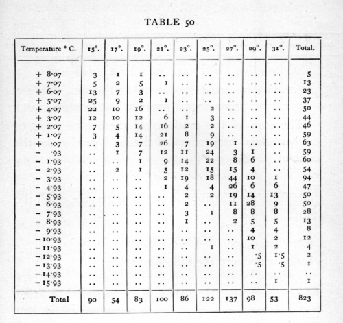
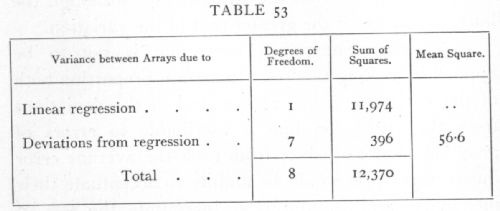
Ex. 42 Test of straightness of regression line. -- The following data are taken from a paper by A. H. Hersh (Journal of Experimental Zoology, xxxix. p. 62) on the influence of temperature on the number of eye facets in Drosophila melanogaster, in various homozygous and heterozygous phases of the "bar" factor. They represent females heterozygous for "full" and "ultra-bar," the facet number being measured in factorial units, effectively a logarithmic scale. Can the influence of temperature on facet number be represented by a straight line, in these units? [p. 215]

There are 9 arrays representing 9 different temperatures. Taking a working mean at -1.93 we calculate the total and average excess over the working mean from each array, and for the aggregate of all 9. Each average is found by dividing the total excess by the number in the array; three decimal places are sufficient save in the aggregate, where four are needed. We have [p. 216]

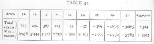
The sum of the products of these nine pairs of numbers, less the product of the final pair, gives the value of

S{n_p(y[bar]_p-y[bar])²} = 12,370,

while from the distribution of the aggregate of all the values of y we have

S(y-y[bar])² = 16,202,

whence is deduced the following table:

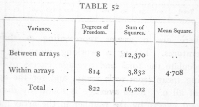
The variance within the arrays is thus only about 4.7; the variance between the arrays will be made up of a part which can be represented by a linear regression, and of a part which represents the deviations of the observed means of arrays from a straight line. To [p. 217]

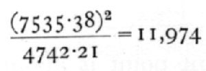
find the part represented by a linear regression, calculate

S(x-x[bar])² = 4742.21

and

S(x-x[bar])(y-y[bar]) = -7535.38,

which latter can be obtained by multiplying the above total excess values by x-x[bar]; then since

we may complete the analysis as follows:

It is useful to check the figure, 396, found by differences, by calculating the actual value of Y for the regression formula and evaluating

S{n_p(y[bar]_p - Y_p)²};

such a check has the advantage that it shows to which arrays in particular the bulk of the discrepancy is due, in this case to the observations at 23 and 25°C.

The deviations from linear regression are evidently larger than would be expected, if the regression were really linear, from the variations within the arrays. For the value of z, we have [p. 218]

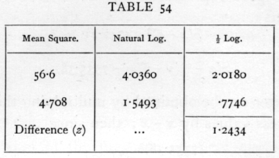
while the 5 per cent point is about .35. There can therefore be no question of the statistical significance of the deviations from the straight line, although the latter accounts for the greater part of the variation.

Note that Sheppard's correction is not to be applied in making this test; a certain proportion both of the variation within arrays, and of the deviations from the regression line is ascribable to errors of grouping, but to deduct from each the average error due to this cause would be unduly to accentuate their inequality, and so to render inaccurate the test of significance.

We have seen how, from the sum of the squares of the deviations of all observations from the general mean, a portion may be separated representing the differences between different arrays. The ratio which this bears to the whole is often denoted by the symbol h², so that

h² = S{n_p(y[bar]_p-y[bar])²} / S(y-y[bar])²,

and the square root of this ratio, h, is called the correlation [p. 219] ratio of y on x. Similarly if Y is the hypothetical regression function, we may define R, so that

R² = S{n_p(Y-y[bar])²} / S(y-y[bar])²,

then R will be the correlation coefficient between y and Y, and if the regression is linear, R² = r², where r is the correlation coefficient between x and y. From these relations it is obvious that h exceeds R, and thus that h provides an upper limit, such that no regression function can be found, the correlation of which with y is higher than h.

As a descriptive statistic the utility of the correlation ratio is extremely limited. It will be noticed that the number of degrees of freedom in the numerator of h² depends on the number of the arrays, so that, for instance in Example 42, the value of h obtained will depend, not only on the range of temperatures explored, but on the number of temperatures employed within a given range.

To test if an observed value of the correlation ratio is significant is to test if the variation between arrays is significantly greater than is to be expected without correlation, from the variation within arrays, and this can be done from the analysis of variance (Table 52) by means of the table of z. Attempts have been made to test the significance of the correlation ratio by calculating for it a standard error, but such attempts overlook the fact that, even with indefinitely large samples, the distribution of h for zero correlation does not tend to normality, unless the number of arrays also is increased without limit. On the contrary, [p. 220] with very large samples, when N is the total number of observations, Nh² tends to be distributed as is c² when n, the number of degrees of freedom, is equal to (a-1).·

In the same sense that ·h² measures the difference between different arrays, so h²-R² measures the aggregate deviation of the means of the arrays from the hypothetical regression line. The attempt to obtain a criterion of linearity of regression by comparing this quantity to its standard error, results in the test known as Blakeman's criterion. In this test, also, no account is taken of the number of the arrays, and in consequence it does not provide even a first approximation in estimating what values of h²-r² are permissible. Similarly with h with zero correlation, so with h²-r², the correlation being linear, if the number of observations is increased without limit, the distribution does not tend to normality, but that of N(h²-r²) tends to be distributed as is c² when n=a-2. Its mean value is then (a-2), and to ignore the value of a is to disregard the main feature of its sampling distribution.

In Example 42 we have seen that with 9 arrays the departure from linearity was very markedly significant; it is easy to see that had there been go arrays, with the same values of h² and r², the departure from linearity would have been even less than the expectation based on the variation within each array. Using Blakeman's criterion, however, these two opposite conditions are indistinguishable. [p. 221]

As in other cases of testing goodness of fit, so in testing regression lines it is essential that if any parameters have to be fitted to the observations, this process of fitting shall have been efficiently carried out.

Some account of efficient methods has been given in Chapter V. In general, save in the more complicated cases, of which this book does not treat, the necessary condition may be fulfilled by the procedure known as the Method of Least Squares, by which the measure of deviation

S{n_p(y[bar]_p-Y_p)²}

is reduced to a minimum subject to the hypothetical conditions which govern the form of Y.

If, as in Section 29 (p. 130), the regression of a dependent variate y on a number of independent variates x₁, x₂, x₃, is expressed in the form

Y = b₁x₁ + b₂x₂ + b₃x₃

then the correlation between y and Y is greater than the correlation of y with any other linear function of the independent variates, and thus measures, in a sense, the extent to which the value of y depends upon, or is related to, the combined variation of these variates. The value of the correlation so obtained, denoted by R, may be calculated from the formula

R² = {b₁S(x₁y) + b₂S(x₂y) + b₃S(x₃y)} / S(y²)

The multiple correlation, R, differs from the correlation obtained with a single independent variate in that it is always positive; moreover it has been recognised [p. 222] in the case of the multiple correlation that its random sampling distribution must depend on the number of independent variates employed. The case is in fact strictly comparable with that of the correlation ratio, and may be accurately treated by means of a table of the analysis of variance.

In the section referred to we made use of the fact that

S(y²) = S(y-Y)² + {b₁S(x₁y) + b₂S(x₂y) + b₃S(x₃y)}

if n' is the number of observations of y, and p the number of independent variates, these three terms will represent respectively n'-1, n'-p-1, and p degrees of freedom. Consequently the analysis of variance takes the form:

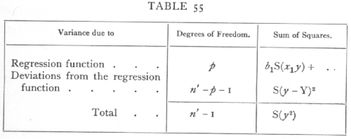
it being assumed that y is measured from its mean value.

If in reality there is no connexion between the independent variates and the dependent variate y, the values in the column headed "sum of squares" will be divided approximately in proportion to the number of degrees of freedom; whereas if a significant connexion exists, then the p degrees of freedom in the [p. 223] regression function will obtain distinctly more than their share. The test, whether R is or is not significant, is in fact exactly the test whether the mean square ascribable to the regression function is or is not significantly greater than the mean square of deviations from the regression function, and may be carried out, as in all such cases, by means of the table of z.

Ex. 43. Significance of a multiple correlation. -- To illustrate the process we may perform the test whether the rainfall data of Example 23 was significantly related to the longitude, latitude, and altitude of the recording stations. From the values found in that example, the following table may be immediately constructed.

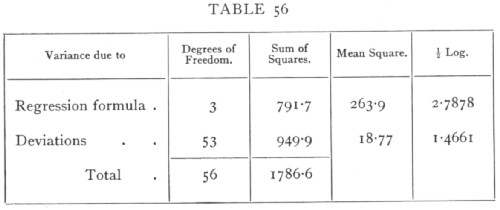
The value of z is thus 1.3217 while the 5 per cent point is about .4415, showing that the multiple correlation is clearly significant. The actual value of the multiple correlation may easily be calculated from the above table, for

R² =791.7 / 1786.6 = .4431

R = .6657;

but this step is not necessary in testing the significance. [p. 224]

The statistical procedure of the analysis of variance is essential to an understanding of the principles underlying modern methods of arranging field experiments. The first requirement which governs all well-planned experiments is that the experiment should yield not only a comparison of different manures, treatments, varieties, etc., but also a means of testing the significance of such differences as are observed. Consequently all treatments must at least be duplicated, and preferably further replicated, in order that a comparison of replicates may be used as a standard with which to compare the observed differences. This is a requirement common to most types of experimentation; the peculiarity of agricultural field experiments lies in the fact, verified in all careful uniformity trials, that the area of ground chosen for the experimental plots may be assumed to be markedly heterogeneous, in that its fertility varies in a systematic, and often a complicated manner from point to point. For our test of significance to be valid the difference in fertility between plots chosen as parallels must be truly representative of the differences between plots with different treatment; and we cannot assume that this is the case if our plots have been chosen in any way according to a pre-arranged system; for the systematic arrangement of our plots may have, and tests with the results of uniformity trials show that it often does have, features in common with the systematic variation of fertility, and thus the test of significance is wholly vitiated. [p. 225]

Ex. 44. Accuracy attained by random arrangement. -- The direct way of overcoming this difficulty is to arrange the plots wholly at random. For example, if 20 strips of land were to be used to test 5 different treatments each in quadruplicate, we might take such an arrangement as the following, found by shuffling 20 cards thoroughly and setting them out in order:

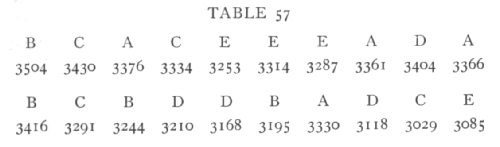
The letters represent 5 different treatments; beneath each is shown the weight of mangold roots obtained by Mercer and Hall in a uniformity trial with 20 such strips.

The deviations in the total yield of each treatment are

in the analysis of variance the sum of squares corresponding to "treatment" will be the sum of these squares divided by 4. Since the sum of the squares of the 20 deviations from the general mean is 289,766, we have the following analysis: [p. 226]

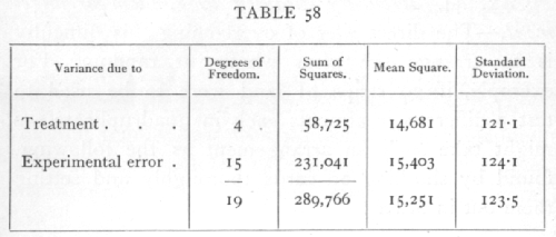
It will be seen that the standard error of a single plot estimated from such an arrangement is 124.1, whereas, in this case, we know its true value to be 223.5; this is an exceedingly close agreement, and illustrates the manner in which a purely random arrangement of plots ensures that the experimental error calculated shall be an unbiassed estimate of the errors actually present.

Ex. 45. Restrictions upon random arrangement. -- While adhering to the essential condition that the errors by which the observed values are affected shall be a random sample of the errors which contribute to our estimate of experimental error, it is still possible to eliminate much of the effect of soil heterogeneity, and so increase the accuracy of our observations by laying restrictions on the order in which the strips are arranged. As an illustration of a method which is widely applicable, we may divide the 20 strips into 5 blocks, and impose the condition that each treatment shall occur once in each block; we shall then be able to separate the variance into three parts representing (i.) local differences between blocks, (ii.) [p. 227] differences due to treatment, (iii.) experimental errors; and if the five treatments are arranged at random within each block, our estimate of experimental error will be an unbiassed estimate of the actual errors in the differences due to treatment. As an example of a random arrangement subject to the above restriction, the following was obtained:

A E C D B  |  C B E D A  |  A D E B C  |  C E B A D.

Analysing out, with the same data as before, the contributions of local differences between blocks, and of treatment, we find

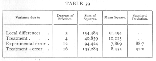
The local differences between the blocks are very significant, so that the accuracy of our comparisons is much improved, in fact the remaining variance is reduced almost to 55 per cent of its previous value. The arrangement arrived at by chance has happened to be a slightly unfavourable one, the errors in the treatment values being a little more than usual, while the estimate of the standard error is 88.7 against a true value 92.0. Such variation is to be expected, and indeed upon it is our calculation of significance based. [p. 228]

It might have been thought preferable to arrange the experiment in a systematic order, such as

and, as a matter of fact, owing to the marked fertility gradient exhibited by the yields in the present example, such an arrangement would have produced smaller errors in the totals of the four treatments. With such an arrangement, however, we have no guarantee that an estimate of the standard error derived from the discrepancies between parallel plots is really representative of the differences produced between the different treatments, consequently no such estimate of the standard error can be trusted, and no test of significance is possible. A more promising way of eliminating that part of the fertility gradient which is not included in the differences between blocks, would be to impose the restriction that each treatment should be "balanced" in respect to position within the block. Thus if any treatment occupied in one block the first strip, in another block the third strip, and in the two remaining blocks the fourth strip (the ordinal numbers adding up to 12), its positions in the blocks would be balanced, and the total yield would be unaffected by the fertility gradient. Of the many arrangements possible subject to this restriction one could be chosen, and one additional degree of freedom eliminated, representing the variance due to average fertility gradient within the blocks. In the present data, where the fertility gradient is large, this would seem to [p. 229] give a great increase in accuracy, the standard error so estimated being reduced from 92.0 to 73.4. But upon examination it appears that such an estimate is not genuinely representative of the errors by which the comparisons are affected, and we shall not thus obtain a reliable test of significance.

The method of laying restrictions on the distribution of the plots and eliminating the corresponding degrees of freedom from the variance is, however, capable of some extension in suitably planned experiments. In a block of 25 plots arranged in 5 rows and 5 columns, to be used for testing 5 treatments, we can arrange that each treatment occurs once in each row, and also once in each column, while allowing free scope to chance in the distribution subject to these restrictions. Then out of the 24 degrees of freedom, 4 will represent treatment; 8 representing soil differences between different rows or columns, may be eliminated; and 12 will remain for the estimation of error. These 12 will provide an unbiassed estimate of the errors in the comparison of treatments provided that every pair of plots, not in the same row or column, belong equally frequently to the same treatment.

Ex. 46. Doubly restricted arrangements. -- The following root weights for mangolds were found by Mercer and Hall in 25 plots; we have distributed letters representing 5 different treatments in such a way that each appears once is each row and column. [p. 230]

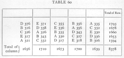
Analysing out the contributions of rows, columns, and treatments we have

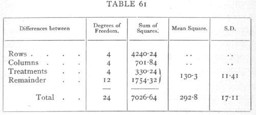
By eliminating the soil differences between different rows and columns, the mean square has been reduced to less than half, and the value of the experiment as a means of detecting differences due to treatment is therefore more than doubled. This method of equalising the rows and columns may with advantage be combined with that of equalising the distribution over different blocks of land, so that very accurate results may be obtained by using a number of blocks each [p. 231] arranged in, for example, 5 rows and columns. In this way the method may be applied even to cases with only three treatments to be compared. Further, since the method is suitable whatever may be the differences in actual fertility of the soil, the same statistical method of reduction may be used when, for instance, the plots are 25 strips lying side by side. Treating each block of five strips in turn as though they were successive columns in the former arrangement, we may eliminate, not only the difference between the blocks, but such differences as those due to a fertility gradient, which affect the yield according to the order of the strips in the block. When, therefore, the number of strips employed is the square of the number of treatments, each treatment can be not only balanced but completely equalised in respect to order in the block, and we may rely upon the (usually) reduced value of the standard error obtained by eliminating the corresponding degrees of freedom. Such a double elimination may be especially fruitful if the blocks of strips coincide with some physical feature of the field such as the ploughman's "lands," which often produce a characteristic periodicity in fertility due to variations in depth of soil, drainage, and such factors.

To sum up: systematic arrangements of plots in field trials should be avoided, since with these it is usually possible to estimate the experimental error in several different ways, giving widely different results, each way depending on some one set of assumptions as to the distribution of natural fertility, which may or may not be justified. With unrestricted random [p. 232] arrangement of plots the experimental error, though accurately estimated, will usually be unnecessarily large. In a well-planned experiment certain restrictions may be imposed upon the random arrangement of the plots in such a way that the experimental error may still be accurately estimated, while the greater part of the influence of soil heterogeneity may be eliminated.

It may be noted that when, by an improved method of arranging the plots, we can reduce the standard error to one-half, the value of the experiment is increased at least fourfold; for only by repeating the experiment four times in its original form could the same accuracy have been attained. This argument really underestimates the preponderance in the scientific value of the more accurate experiments, for, in agricultural plot work, the experiment cannot in practice be repeated upon identical climatic and soil conditions.