Classics in the History of Psychology

An internet resource developed by
Christopher D. Green
York University, Toronto, Ontario
ISSN 1492-3173

(Return to index)

STATISTICAL METHODS FOR RESEARCH WORKERS

The fundamental proposition upon which the statistical treatment of mean values is based is that -- If a quantity be normally distributed with standard deviation s, then the mean of a random sample of n such quantities is normally distributed with standard deviation s/[sqrt]n.

The utility of this proposition is somewhat increased by the fact that even if the original distribution were not exactly normal, that of the mean usually tends to normality, as the size of the sample is increased; the method is therefore applied widely and legitimately to cases in which we have not sufficient evidence to assert that the original distribution was normal, but in which we have reason to think that it does not belong to the exceptional class of distributions for which the distribution of the mean does not tend to normality.

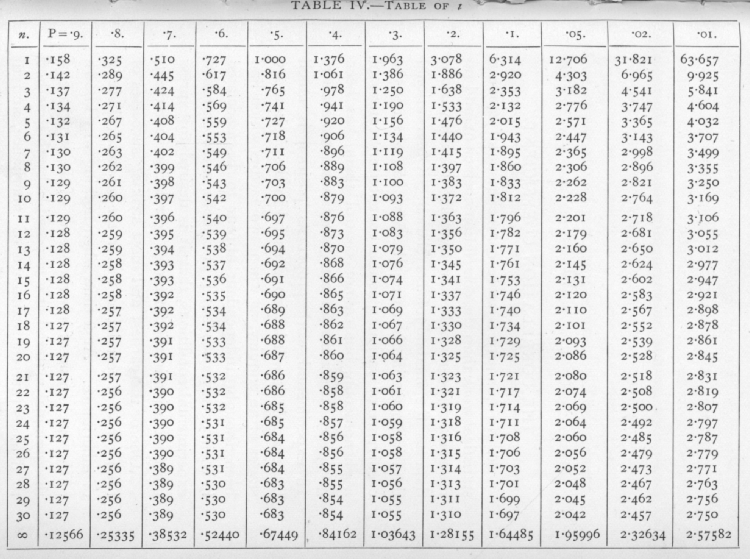
If, therefore, we know the standard deviation of a population, we can calculate the standard deviation of [p. 102] the mean of a random sample of any size, and so test whether or not it differs significantly from any fixed value. If the difference is many times greater than the standard error, it is certainly significant, and it is a convenient convention to take twice the standard error as the limit of significance ; this is roughly equivalent to the corresponding limit P=.05, already used for the c² distribution. The deviations in the normal distribution corresponding to a number of values of P are given in the lowest line of the table of t at the end of this chapter (p. 137)· More detailed information has been given in Table I.

Ex. 16. Significance of mean of a large sample. -- We may consider from this point of view Weldon's die-casting experiment (Ex. 5, p. 66). The variable quantity is the number of dice scoring "5" or "6" in a throw of 12 dice. In the experiment this number varies from zero to eleven, with an observed mean of 4.0524; the expected mean, on the hypothesis that the dice were true, is 4, so that the deviation observed is .0524· If now we estimate the variance of the whole sample of 26,306 values as explained on p. 50, but without using Sheppard's correction (for the data are not grouped), we find

s² = 2.69825,

whence s²/n = .0001025,

and s/[sqrt]n = .01013.

The standard error of the mean is therefore about .01, and the observed deviation is nearly 5.2 times as great; thus by a slightly different path we arrive [p. 103] at the same conclusion as that of p. 68. The difference between the two methods is that our treatment of the mean does not depend upon the hypothesis that the distribution is of the binomial form, but on the other hand we do assume the correctness of the value of s derived from the observations. This assumption breaks down for small samples, and the principal purpose of this chapter is to show how accurate allowance can be made in these tests of significance for the errors in our estimates of the standard deviation.

To return to the cruder theory, we may often, as in the above example, wish to compare the observed mean with the value appropriate to a hypothesis which we wish to test; but equally or more often we wish to compare two experimental values and to test their agreement. In such cases we require the standard error of the difference between two quantities whose standard errors are known; to find this we make use of the proposition that the variance of the difference of two independent variates is equal to the sum of their variances. Thus, if the standard deviations are s₁, s₂, the variances are s₁², s₂²; consequently the variance of the difference is s₁²+s₂², and the standard error of the difference is [sqrt]s₁²+s₂².

Ex. 17· Standard error of difference of means from large samples. -- In Table 2 is given the distribution in stature of a group of men, and also of a group of women; the means are 68.64 and 63.85 inches, giving a difference of 4.79 inches. The variance obtained for the men was 7.2964 square inches; this is the value obtained by dividing the sum of the squares of [p. 104] the deviations by 1164 ; if we had divided by 1163, to make the method comparable to that appropriate to small samples, we should have found 7.3027. Dividing this by 1164, we find the variance of the mean is .006274. Similarly the variance for the women is .63125, which divided by 1456 gives the variance of the mean of the women as .004335. To find the variance of the difference between the means, we must add together these two contributions, and find in all .010609; the standard error of the difference between the means is therefore .1030 inches. The sex difference in stature may therefore be expressed as

4.79 [plus or minus] .103 inches.

It is manifest that this difference is significant, the value found being over 46 times its standard error. In this case we can not only assert a significant difference, but place its value with some confidence at between 4½ and 5 inches. It should be noted that we have treated the two samples as independent, as though they had been given by different authorities; as a matter of fact, in many cases brothers and sisters appeared in the two groups; since brothers and sisters tend to be alike in stature, we have overestimated the probable error of our estimate of the sex difference. Whenever possible, advantage should be taken of such facts in designing experiments. In the common phrase, sisters provide a better "control" for their brothers than do unrelated women. The sex difference could therefore be more accurately estimated from the comparison of each brother with his own sister. In [p. 105] the following example (Pearson and Lee's data), taken from a correlation table of stature of brothers and sisters, the material is nearly of this form; it differs from it in that in some instances the same individual has been compared with more than one sister, or brother.

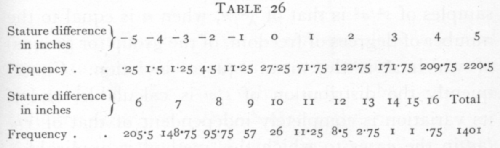
Ex. I8. Standard error of mean of differences. -- The following table gives the distribution of the excess in stature of a brother over his sister in 1401 pairs

Treating this distribution as before we obtain: mean=4.895, variance=6.4074, variance of mean=.004573, standard error of mean =.0676 ; showing that we may estimate the mean sex difference as 4¾ to to 5 inches.

In the above examples, which are typical of the use of the standard error applied to mean values, we have assumed that the variance of the population is known with exactitude. It was pointed out by "Student" in 1908, that with small samples, such as are of necessity usual in field and laboratory experiments, the variance of the population can only be roughly estimated from the sample, and that the errors of estimation seriously affect the use of the standard error. [p. 106]

If x (for example the mean of a sample) is a value with normal distribution and s is its true standard error, then the probability that x/s exceeds any specified value may be obtained from the appropriate table of the normal distribution; but if we do not know s, but in its place have s, an estimate of the value of s,the distribution required will be that of x/s, and this is not normal. The true value has been divided by a factor, s/s, which introduces an error. We have seen in the last chapter that the distribution in random samples of s²/s² is that of c²/n, when n is equal to the number of degrees of freedom, of the group (or groups) of which s² is the mean square deviation. Consequently the distribution of s/s calculable, and if its variation is completely independent of that of x/s (as in the cases to which this method is applicable), then the true distribution of x/s can be calculated, and accurate allowance made for its departure from normality. The only modification required in these cases depends solely on the number n, representing the number of degrees of freedom available for the estimation of s. The necessary distributions were given by "Student" in 1908; fuller tables have since been given by the same author, and at the end of this chapter (p. 137) we give the distributions in a similar form to that used for our table of c².

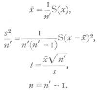
If x₁, x₂, ..., x_n, is a sample of n' values of a variate, x, and if this sample constitutes the whole of [p. 107] the information available on the point in question, then we may test whether the mean of x differs significantly from zero, by calculating the statistics

The distribution of t for random samples of a normal population distributed about zero as mean, is given in the table of t for each value of n. The successive columns show, for each value of n, the values of t for which P, the probability of falling outside the range [plus or minus]t, takes the values .9,...,.01, at the head of the columns. Thus the last column shows that, when n=10, just I per cent of such random samples will give values of t exceeding +3.169, or less than -3.169. If it is proposed to consider the chance of exceeding the given values of t, in a positive (or negative) direction only, then the values of P should be halved. It will be seen from the table that for any degree of certainty we require higher values of t, the smaller the value of n. The bottom line of the table, corresponding to infinite values of n, gives the values of a normally distributed variate, in terms of its standard deviation, for the same values of P.

Ex. 19. Significance of mean of a small sample. -- The following figures (Cushny and Peebles' data) [p. 108] which I quote from Student's paper show the result of an experiment with ten patients, on the effect of the optical isomers of hyoscyamine hydrobromide in producing sleep.

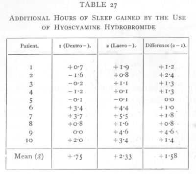
The last column gives a controlled comparison of the efficacy of the two drugs as soporifics, for the same patients were used to test each; from the series of differences we find

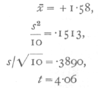
For n=9, only one value in a hundred will exceed 3250 by chance, so that the difference between the results is clearly significant. By the methods of the [p. 109] previous chapters we should, in this case, have been led to the same conclusion with almost equal certainty; for if the two drugs had been equally effective, positive and negative signs would occur in the last column with equal frequency. Of the 9 values other than zero, however, all are positive, and it appears from the binomial distribution,

(½+½)⁹,

that all will be of the same sign, by chance, only twice in 512 trials. The method of the present chapter differs from that in taking account of the actual values and not merely of their signs, and is consequently the more reliable method when the actual values are available.

To test whether two samples belong to the same population, or differ significantly in their means. If x'₁, x'₂,…,x'_n1+1, and If x₁, x₂,…,x_n2+1 be two samples, the significance of the difference between their means may be tested by calculating the following statistics.

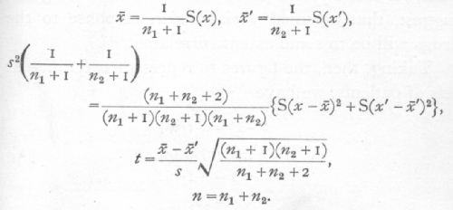
The means are calculated as usual; the standard [p. 110] deviation is estimated by pooling the sums of squares from the two samples and dividing by the total number of the degrees of freedom contributed by them; if a were the true standard deviation, the variance of the first mean would be s²/(n₁+1), of the second mean s²/(n₂+1), and therefore of the difference s²{1/(n₁+1)+1/(n₂+1)}; t is therefore found by dividing x[bar]-x'[bar] by its standard error as estimated, and the error of the estimation is allowed for by entering the table with n equal to the number of degrees of freedom available for estimating s; that is n=n₁+n₂. It is thus possible to extend Student's treatment of the error of a -an to the comparison of the means of two samples.

Ex. 20. Significance of difference of means of small samples. -- Let us suppose that the above figures (Table 27) had been obtained using different patients for the two drugs; the experiment would have been less well controlled, and we should expect to obtain less certain results from the same number of observations, for it is a priori probable, and the above figures suggest, that personal variations in response to the drugs will be to some extent correlated.

Taking, then, the figures to represent two different sets of patients, we have

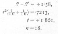
The value of P is, therefore, between .1 and .05, and [p. 111] cannot be regarded as significant. This example shows clearly the value of design in small scale experiments, and that the efficacy of such design is capable of statistical measurement.

The use of Student's distribution enables us to appreciate the value of observing a sufficient number of parallel cases; their value lies, not only in the fact that the probable error of a mean decreases inversely as the square root of the number of parallels, but in the fact that the accuracy of our estimate of the probable error increases simultaneously. The need for duplicate experiments is sufficiently widely realised; it is not so widely understood that in some cases, when it is desired to place a high degree of confidence (say P =.01) on the results, triplicate experiments will enable us to detect with confidence differences as small as one-seventh of those which, with a duplicate experiment, would justify the same degree of confidence.

The confidence to be placed in a result depends not only on the actual value of the mean value obtained, but equally on the agreement between parallel experiments. Thus, if in an agricultural experiment a first trial shows an apparent advantage of 8 tons to the acre, and a duplicate experiment shows an advantage of 9 tons, we have n=1, t=17, and the results would justify some confidence that a real effect had been observed; but if the second experiment had shown an apparent advantage of 18 tons, although the mean is now higher, we should place not more but less confidence in the conclusion that the treatment was [p. 112] beneficial, for t has fallen to 2.6, a value which for n=1 is often exceeded by chance. The apparent paradox may be explained by pointing out that the difference of 10 tons between the experiments indicates the existence of uncontrolled circumstances so influential that in both cases the apparent benefit may be due to chance, whereas in the former case the relatively close agreement of the results suggests that the uncontrolled factors are not so very influential. Much of the advantage of further replication lies in the fact that with duplicates our estimate of the importance of the uncontrolled factors is so extremely hazardous.

In cases in which each observation of one series corresponds in some respects to a particular observation of the second series, it is always legitimate to take the differences and test them as in Ex. 18, 19 as a single sample; but it is not always desirable to do so. A more precise comparison is obtainable by this method only if the corresponding values of the two series are positively correlated, and only if they are correlated to a sufficient extent to counterbalance the loss of precision due to basing our estimate of variance upon fewer degrees of freedom. An example will make this plain.

Ex. 21. Significance of change in bacterial numbers. -- The following table shows the mean number of bacterial colonies per plate obtained by four slightly different methods from soil samples taken at 4 P.M. and 8 P.M. respectively (H. G. Thornton's data): [p. 113]

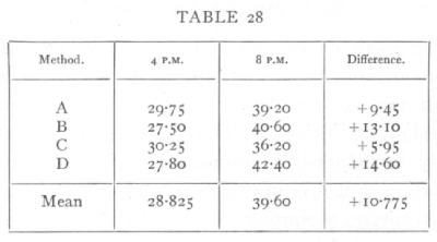
From the series of differences we have x[bar]=+10.775, ¼s²=3.756, t=5.560, n=3, whence the table shows that P is between .01 and .02. If, On the contrary, we use the method of Ex. 20, and treat the two separate series, we find x[bar]-x'[bar]=+10.775, ½s²=2.188, t =7.285, n=6; this is not only a larger value of n but a larger value of t, which is now far beyond the range of the table, showing that P is extremely small. In this case the differential effects of the different methods are either negligible, or have acted quite differently in the two series, so that precision was lost in comparing each value with its counterpart in the other series. In cases like this it sometimes occurs that one method shows no significant difference, while the other brings it out; if either method indicates a definitely significant difference, its testimony cannot be ignored, even if the other method fails to show the effect. When no correspondence exists between the members of one series and those of the other, the second method only is available. [p. 114]

The methods of this chapter are applicable not only to mean values, in the strict sense of the word, but to the very wide class of statistics known as regression coefficients. The idea of regression is usually introduced in connection with the theory of correlation, but it is in reality a more general, and, in some respects, a simpler idea, and the regression co-efficients are of interest and scientific importance in many classes of data where the correlation coefficient, if used at all, is an artificial concept of no real utility. The following qualitative examples are intended to familiarise the student with the concept of regression, and to prepare the way for the accurate treatment of numerical examples.

It is a commonplace that the height of a child depends on his age, although knowing his age, we cannot accurately calculate his height. At each age the heights are scattered over a considerable range in a frequency distribution characteristic of that age; any feature of this distribution, such as the mean, will be a continuous function of age. The function which represents the mean height at any age is termed the regression function of height on age; it is represented graphically by a regression curve, or regression line. In relation to such a regression line age is termed the independent variate, and height the dependent variate.

The two variates bear very different relations to the regression line. If errors occur in the heights, this [p. 115] will not influence the regression of height on age, provided that at all ages positive and negative errors are equally frequent, so that they balance in the averages. On the contrary, errors in age will in general alter the regression of height on age, so that from a record with ages subject to error, or classified in broad age-groups, we should not obtain the true physical relationship between mean height and age. A second difference should be noted: the regression function does not depend on the frequency distribution of the independent variate, so that a true regression line may be obtained even when the age groups are arbitrarily selected, as when an investigation deals with children of "school age." On the other hand a selection of the dependent variate will change the regression line altogether.

It is clear from the above instances that the regression of height on age is quite different from the regression of age on height; and that one may have a definite physical meaning in cases in which the other has only the conventional meaning given to it by mathematical definition. In certain cases both regressions are of equal standing; thus, if we express in terms of the height of the father the average adult height of sons of fathers of a given height, observation shows that each additional inch of the fathers' height corresponds to about half an inch in the mean height of the sons. Equally, if we take the mean height of the fathers of sons of a given height, we find that each additional inch of the sons' height corresponds to half an inch in the mean height of the fathers. No selection [p. 116] has been exercised in the heights either of fathers or of sons; each variate is distributed normally, and the aggregate of pairs of values forms a normal correlation surface. Both regression lines are straight, and it is consequently possible to express the facts of regression in the simple rules stated above.

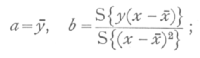
When the regression line with which we are concerned is straight, or, in other words, when the regression function is linear, the specification of regression is much simplified, for in addition to the general means we have only to state the ratio which the increment of the mean of the dependent variate bears to the corresponding increment of the independent variate. Such ratios are termed regression coefficients. The regression function takes the form

Y = a+b(x-x[bar]),

where b is the regression coefficient of y on x, and Y is the mean value of y for each value of x. The physical dimensions of the regression coefficient depend on those of the variates; thus, over an age range in which growth is uniform we might express the regression of height on age in inches per annum, in fact as an average growth rate, while the regression of father's height on son's height is half an inch per inch, or simply ½. Regression coefficients may, of course, be positive or negative.

Curved regression lines are of common occurrence ; in such cases we may have to use such a regression function as

Y = a+bx+cx²+dx³, [p. 117]

in which all four coefficients of the regression function may, by an extended use of the term, be called regression coefficients. More elaborate functions of x may be used, but their practical employment offers difficulties in cases where we lack theoretical guidance in choosing the form of the regression function, and at present the simple power series (or, polynomial in x) is alone in frequent use. By far the most important case in statistical practice is the straight regression line.

The straight regression line with formula

Y = a+b(x-x[bar])

is fitted by calculating from the data, the two statistics

these are estimates, derived from the data, of the two constants necessary to specify the straight line; the true regression formula, which we should obtain from an infinity of observations, may be represented by

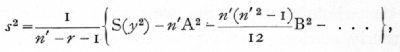
a+b(x-x[bar]),

and the differences a-a, b-b, are the errors of random sampling of our statistics. If s² represent the variance of y for any value of x about a mean given by the above formula, then the variance of a, the mean of n' observations, will be s²/n', while that of b, which is [p. 118] merely a weighted mean of the values of y observed, will be

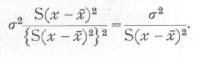
In order to test the significance of the difference between b, and any hypothetical value, b, to which it is to be compared, we must estimate the value of s²; the best estimate for the purpose is

found by summing the squares of the deviations of y from its calculated value Y, and dividing by (n'-2). The reason that the divisor is (n'-2) is that from the n' values of y two statistics have already been calculated which enter into the formula for Y, consequently the group of differences, y-Y, represent in reality only n'-2 degrees of freedom.

When n' is small, the estimate of s² obtained above is somewhat uncertain, and in comparing the difference b-b with its standard error, in order to test its significance we shall have to use Student's method, with n=n'-2. When n' is large this distribution tends to the normal distribution. The value of t with which the table must be entered is

Similarly, to test the significance of the difference between a and any hypothetical value a, the table is entered with [p. 119]

this test for the significance of a will be more sensitive than the method previously explained, if the variation in y is to any considerable extent expressible in terms of that of x, for the value of s obtained from the regression line will then be smaller than that obtained from the original group of observations. On the other hand, one degree of freedom is always lost, so that if b is small, no greater precision is obtained.

Ex. 22. Effect of nitrogenous fertilisers in maintaining yield. -- The yields of dressed grain in bushels per acre shown in Table 29 were obtained from two plots on Broadbalk wheat field during thirty years; the only difference in manurial treatment was that "9a" received nitrate of soda, while "7b" received an equivalent quantity of nitrogen as sulphate of ammonia. In the course of the experiment plot "9a" appears to be gaining in yield on plot "7b." Is this apparent gain significant?

A great part of the variation in yield from year to year is evidently similar in the two plots; in consequence, the series of differences will give the clearer result. In one respect the above data are especially simple, for the thirty values of the independent variate form a series with equal intervals between the successive values, with only one value of the dependent variate corresponding to each. In such cases the work is simplified by using the formula

S(x-x[bar])² = 1/12 n' (n'²-1), [p. 120]

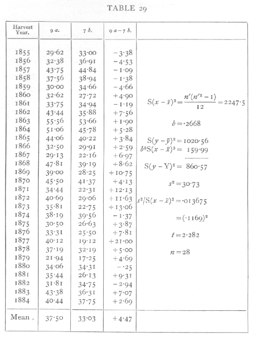
where n' is the number of terms, or 30 in this case. To evaluate 6 it is necessary to calculate

S{y(x-x[bar])};

this may be done in several ways. We may multiply [p. 121] the successive values of y by -29, -27,… +27, +29, add, and divide by 2. This is the direct method suggested by the formula. The same result is obtained by multiplying by 1, 2, ..., 30 and subtracting 15½ times the sum of values of y; the latter method may be conveniently carried out by successive addition. Starting from the bottom of the column, the successive sums 2.69, 9.76, 6.82, ... are written down, each being found by adding a new value of y to the total already accumulated; the sum of the new column, less 15½ times the sum of the previous column, will be the value required. In this case we find the value 599.615, and dividing by 2247.5, the value of b is found to be .2668. The yield of plot "9a" thus appears to have gained on that of "7b" at a rate somewhat over a quarter of a bushel per annum.

To estimate the standard error of 6, we require the value of

S(y-Y)²;

knowing the value of b, it is easy to calculate the thirty values of Y from the formula

Y =y[bar]+(x-x[bar])b;

for the first value, x-x[bar]=-14.5 and the remaining values may be found in succession by adding b each time. By subtracting each value of Y from the corresponding y, squaring, and adding, the required quantity may be calculated directly. This method is laborious, and it is preferable in practice to utilise the algebraical fact that [p. 122]

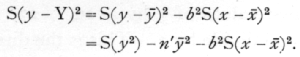
The work then consists in squaring the values of y and adding, then subtracting the two quantities which can be directly calculated from the mean value of y and the value of b. In using this shortened method it should be noted that small errors in y[bar] and b may introduce considerable errors in the result, so that it is necessary to be sure that these are calculated accurately to as many significant figures as are needed in the quantities to be subtracted. Errors of arithmetic which would have little effect in the first method, may altogether vitiate the results if the second method is used. The subsequent work in calculating the standard error of b may best be followed in the scheme given beside the table of data ; the estimated standard error is .1169, so that in testing the hypothesis that b=0 that is that plot "9a" has not been gaining on plot "7b," we divide b by this quantity and find t=2.282. Since s was found from 28 degrees of freedom n=28, and the table of t shows that P is between .02 and .05.·

The result must be judged significant, though barely so; in view of the data we cannot ignore the possibility that on this field, and in conjunction with the other manures used, nitrate of soda has conserved the fertility better than sulphate of ammonia ; these data do not, however, demonstrate the point beyond possibility of doubt.

The standard error of y[bar], calculated from the above data, is 1.012, so that there can be no doubt that the [p. 123] difference in mean yields is significant; if we had tested the significance of the mean, without regard to the order of the values, that is calculating s² by dividing 1020.56 by 29, the standard error would have been 1.083. The value of b was therefore high enough to have reduced the standard error. This suggests the possibility that if we had fitted a more complex regression line to the data the probable errors would be further reduced to an extent which would put the significance of b beyond doubt. We shall deal later with the fitting of curved regression lines to this type of data.

Just as the method of comparison of means is applicable when the samples are of different sizes, by obtaining an estimate of the error by combining the sums of squares obtained from the two different samples, so we may compare regression coefficients when the series of values of the independent variate are not identical; or if they are identical we can ignore the fact in comparing the regression coefficients.

Ex. 23. Comparison of relative growth rate of two cultures of an alga. -- Table 30 shows the logarithm (to the base 10) of the volumes occupied by algal cells on successive days, in parallel cultures, each taken over a period during which the relative growth rate was approximately constant. In culture A nine values are available, and in culture B eight (Dr. M. Bristol-Roach's data).

The method of finding Sy(x-x[bar]) by summation is shown in the second pair of columns: the original values are added up from the bottom, giving successive [p. 124] totals from 6.087 to 43.426; the final value should, of course, tally with the total below the original values. From the sum of the column of totals is subtracted the sum of the original values multiplied by 5 for A and by 4½ for B. The differences are Sy(x-x[bar]); these must be divided by the respective values of S(x-xbar])²,

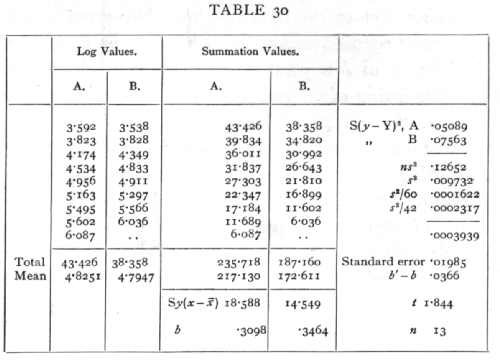
namely, 60 and 42, to give the values of b, measuring the relative growth rates of the two cultures. To test if the difference is significant we calculate in the two cases S(y²), and subtract successively the product of the mean with the total, and the product of b with Sy(x-x[bar]); this process leaves the two values of S(y-Y)², which are added as shown in the table, and the sum divided by n, to give s². The value of n is found by adding the 7 degrees of freedom from series A to the 6 degrees from series B, and is therefore 13. [p. 125] Estimates of the variance of the two regression coefficients are obtained by dividing s² by 60 and 42, and that of the variance of their difference is the sum of these. Taking the square root we find the standard error to be .01985, and t=1.844· The difference between the regression coefficients, though relatively large, cannot be regarded as significant. There is not sufficient evidence to assert culture B was growing more rapidly than culture A.

Little progress has been made with the theory of the fitting of curved regression lines, save in the limited but most important case when the variability of the independent variate is the same for all values of the dependent variate, and is normal for each such value. When this is the case a technique has been fully worked out for fitting by successive stages any line of the form

Y = a+bx+cx²+dx³+.. ;

we shall give details of the case where the successive values of x are at equal intervals.

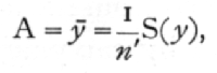
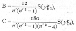
As it stands the above form would be inconvenient in practice, in that the fitting could not be carried through in successive stages. What is required is to obtain successively the mean of y, an equation linear in x, an equation quadratic in x, and so on, each equation being obtained from the last by adding, a new term being calculated by carrying a single process of [p. 126] computation through a new stage. In order to do this we take

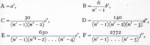
Y = A + Bx₁ + Cx₂ + Dx₃ + …,

where x₁, x₂, x₃, shall be functions of x of the 1st, 2nd, and 3rd degrees, out of which the regression formula may be built. It may be shown that the functions required for this purpose may be expressed in terms of the moments of the x distribution, as follows:

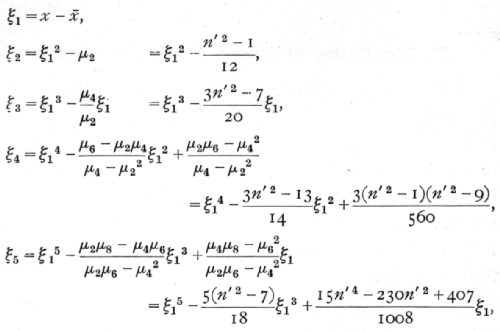
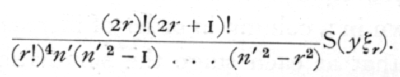
where the values of the moment functions have been expressed in terms of n', the number of observations, as far as is needed for fitting curves up to the 5^th degree. The values of x are taken to increase by unity.

Algebraically the process of fitting may now be represented by the equations

 [p. 127]

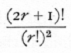
and, in general, the coefficient of the term of the rth degree is

As each term is fitted the regression line approaches more nearly to the observed values, and the sum of the squares of the deviation

S(y-Y)²

is diminished. It is desirable to be able to calculate this quantity, without evaluating the actual values of Y at each point of the series; this can be done by subtracting from S(y²) the successive quantities

and so on. These quantities represent the reduction which the sum of the squares of the residuals suffers each time the regression curve is fitted to a higher degree; and enable its value to be calculated at any stage by a mere extension of the process already used in the preceding examples. To obtain an estimate, s², of the residual variance, we divide by n, the number of degrees of freedom left after fitting, which is found from n' by subtracting from it the number of constants in the regression formula. Thus, if a straight line has been fitted, n=n'-2; while if a curve of the fifth degree has been fitted, n=n'-6. [p. 128]

The main arithmetical labour of fitting curved regression lines to data of this type may be reduced to a repetition of the process of summation illustrated in Ex. 23. We shall assume that the values of y are written down in a column in order of increasing values of x, and that at each stage the summation is commenced at the top of the column (not at the bottom, as in that example). The sums of the successive columns will be denoted by S₁, S₂, ... When these values have been obtained, each is divided by an appropriate divisor, which depends only on n', giving us a new series of quantities a, b, c,... according to the following equations

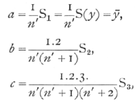
and so on.

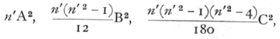
From these a new series of quantities a', b', c',… are obtained by equations independent n', of which we give below the first six, which are enough to carry the process of fitting up to the 5th degree:

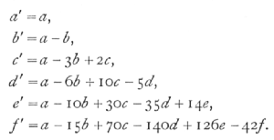 [p. 129]

These new quantities are proportional to the required coefficients of the regression equation, and need only be divided by a second group of divisors to give the actual values. The equations are

the numerical part of the factor being

for the term of degree r.

If an equation of degree r has been fitted, the estimate of the standard errors of the coefficients are all based upon the same value of s², i.e.

from which the estimated standard error of any coefficient, such as that of x_p, is obtained by dividing by

and taking out the square root. The number of degrees of freedom upon which the estimate is based is (n'-r-1), and this must be equated to n in using the table of t.

A suitable example of use of this method may be obtained by fitting the values of Ex. 22 (p. 120) with a curve of the second or third degree. [p. 130]

It frequently happens that the data enable us to express the average value of the dependent variate y, in terms of a number of different independent variates x₁, x₂, … x_p. For example, the rainfall at any point within a district may be recorded at a number of stations for which the longitude, latitude, and altitude are all known. If all of these three variates influence the rainfall, it may be required to ascertain the average effect of each separately. In speaking of longitude, latitude, and altitude as independent variates, all that is implied is that it is in terms of them that the average rainfall is to be expressed; it is not implied that these variates vary independently, in the sense that they are uncorrelated. On the contrary, it may well happen that the more southerly stations lie on the whole more to the west than do the more northerly stations, so that for the stations available longitude measured to the west may be negatively correlated with latitude measure to the north. If, then, rainfall increased to the west but was independent of latitude, we should obtain merely, by comparing the rainfall recorded at different latitudes, a fictitious regression indicating a falling off of rain with increasing latitude. What we require is an equation taking account of all three variates at each station, and agreeing as nearly as possible with the values recorded; this is called a partial regression equation, and its coefficients are known as partial regression coefficients. [p. 131]

To simplify the algebra we shall suppose that y, x₁, x₂, x₃, are all measured from their mean values, and that we are seeking a formula of the form

Y = b₁,x₁+b₂x₂+b₃x₃.

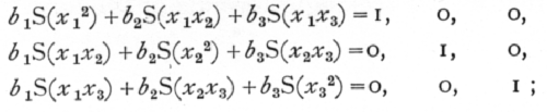
If S stands for summation over all the sets of observations we construct the three equations

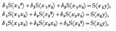
of which the nine coefficients are obtained from the data either by direct multiplication and addition, or, if the data are numerous, by constructing correlation tables for each of the six pairs of variates. The three simultaneous equations for b₁, b₂, and b₃, are solved in the ordinary way; first b₃ is eliminated from the first and third, and from the second and third equations, leaving two equations for b₁ and b₂; eliminating b₂ from these, b₁ is found, and thence by substitution, b₂ and b₃.

It frequently happens that, for the same set of values of the independent variates, it is desired to examine the regressions for more than one set of values of the dependent variates; for example, if for the same set of rainfall stations we had data for several different months or years. In such cases it is preferable to avoid solving the simultaneous equations afresh on each occasion, but to obtain a simpler formula which may be applied to each new case.

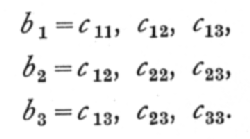
This may be done by solving once and for all the [p. 132] three sets, each consisting of three simultaneous equations:

the three solutions of these three sets of equations may be written

Once the six values of c are known, then the partial regression coefficients may be obtained in any particular case merely by calculating S(x₁y), S(x₂y), S(x₃y) and substituting in the formulæ,

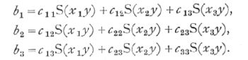
The method of partial regression is of very wide application. It is worth noting that the different independent variates may be related in any way; for example, if we desired to express the rainfall as a linear function of the latitude and longitude, and as a quadratic function of the altitude, the square of the altitude would be introduced as a fourth independent variate, without in any way disturbing the process outlined above, save that S(x₃x₄), S(x₃³) would be calculated directly from the distribution of altitude.

In estimating the sampling errors of partial [p. 133] regression coefficients we require to know how nearly our calculated value, Y, has reproduced the observed values of y; as in previous cases, the sum of the squares of (y-Y) may be calculated by differences, for, with three variates,

S(y-Y)² = S(y²) - b₁S(x₁y) - b₂S(x₂y) - b₃S(x₃y).·

If we had n' observations, and p independent variates, we should therefore find

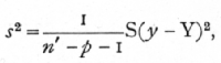
and to test if b₁, differed significantly from any hypothetical value, b₁, we should calculate

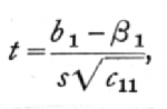
entering the table of t with n=n'-p-1.

In the practical use of a number of variates it is convenient to use cards, on each of which is entered the values of the several variates which may be required. By sorting these cards in suitable grouping units with respect to any two variates the corresponding correlation table may be constructed with little risk of error, and thence the necessary sums of squares and products obtained.

Ex. 24. Dependence of rainfall on position and altitude. -- The situations of 57 rainfall stations in Hertfordshire have a mean longitude 12'.4 W., a mean latitude 51° 48'.5 N., and a mean altitude 302 feet. Taking as units 2 minutes of longitude, one [p. 134] minute of latitude, and 20 feet of altitude, the following values of the sums of squares and products of deviations from the mean were obtained:

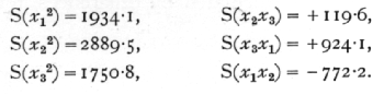
To find the multipliers suitable for any particular set of weather data from these stations, first solve the equations

1934.1 c₁₁ - 772.2 c₁₂ + 924.1 c₁₃ = 1
-772.2 c₁₁ + 2889.5 c₁₂ + 119.6 c₁₃ = 0
+924.1 c₁₁ + 119.6 c_13[sic] + 1750.8 c₁₃ = 0;

using the last equation to eliminate c₁₃ from the first two, we have

2532.3 c₁₁ - 1462.5 c₁₂ = 1.7508
=1462.5 c₁₁ + 5044.6 c₁₂ = 0;

from these eliminate c₁₂, obtaining

10,635.5 c₁₁ = 8.8321;

whence

c₁₁ = .00083043, c₁₂ = .00024075, c₁₃ = -.00045476

the last two being obtained successively by substitution.

Since the corresponding equations for c₁₂, c₂₂, c₂₃ differ only in changes in the right-hand number, we can at once write down

-1462.5 c₁₂ + 5044.6 c₂₂ = 1.7508;

whence, substituting for c₁₂ the value already obtained,

c₂₂ = .00041686, c₂₃ = -.00015554; [p. 135]

finally, to obtain c₃₃ we have only to substitute in the equation

924.1c₁₃ + 119.6c₂₃ + 1750.8c₃₃ = 1,

giving

c₃₃ =.00082182.

It is usually worth while, to facilitate the detection of small errors by checking, to retain as above one more decimal place than the data warrant.

The partial regression of any particular weather data on these three variates can now be found with little labour. In January 1922 the mean rainfall recorded at these stations was 3.87 inches, and the sums of products of deviations with those of the three independent variates were (taking 0.1 inch as the unit for rain)

multiplying these first by c₁₁, c₁₂, c₁₃ and adding, we have for the partial regression on longitude

b₂ = .39624;

similarly using the multipliers c₁₂, c₂₂, c₂₃ we obtain for the partial regression on latitude

b₂ = -11204;

and finally, by using c₁₃, c₂₃, c₃₃,

b₃ = .30787

gives the partial regression on altitude.

Remembering now the units employed, it appears that in the month in question rainfall increased by .0198 of an inch for each minute of longitude westwards, [p. 136] is decreased by .0112 of an inch for each minute of latitude northwards, and increased by .00154 of an inch for each foot of altitude.

Let us calculate to what extent the regression on altitude is affected by sampling errors. For the 57 recorded deviations of the rainfall from its mean value, in the units previously used

S(y²) = 1786.6;

whence, knowing the values of b₁, b₂, and b₃, we obtain by differences

S(y-Y)² = 994.9.

To find s², we must divide this by the number of degrees of freedom remaining after fitting a formula involving three variates -- that is, by 53 -- so that

s² = 8.772;

multiplying this by c₃₃, and taking the square root,

s[sqrt]c₃₃ = .12421.

Since n is as high as 53 we shall not be far wrong in taking the regression of rainfall on altitude to be in working units .308, with a standard error .124; or in inches of rain per 100 feet as .154, with a standard error .062.