Classics in the History of Psychology

An internet resource developed by
Christopher D. Green
York University, Toronto, Ontario
ISSN 1492-3173

(Return to index)

STATISTICAL METHODS FOR RESEARCH WORKERS

In the last chapter some use has been made of the χ² distribution as a means of testing the agreement between observation and hypothesis; in the present chapter we shall deal more generally with the very wide class of problems which may be solved by means of the same distribution.

The common factor underlying all such tests is the comparison of the numbers actually observed to fall into any number of classes with the numbers which upon some hypothesis are expected. If m is the number expected, and m+x the number observed in any class, we calculate

the summation extending over all the classes. This formula gives the value of χ², and it is clear that the more closely the observed numbers agree with those expected the smaller will χ² be; in order to utilise the table it is necessary to know also the value of n with which the table is to be entered. The rule for finding [p. 78] n is that n is equal to the number-of degrees of freedom in which the observed series may differ from the hypothetical; in other words, it is equal to the number of classes the frequencies in which may be filled up arbitrarily. Several examples will be given to illustrate this rule.

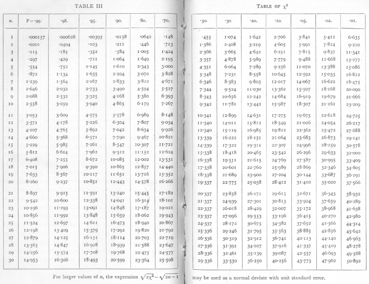
For any value of n, which must be a whole number, the form of distribution of χ² was established by Pearson in 1900; it is therefore possible to calculate in what proportion of cases any value of χ² will be exceeded. This proportion is represented by P, which is therefore the probability that χ² shall exceed any specified value. To every value of χ² there thus corresponds a certain value of P; as χ² is increased from o to infinity, P diminishes from 1 to 0. Equally, to any value of P in this range there corresponds a certain value of χ². Algebraically the relation between these two quantities is a complex one, so that it is necessary to have a table of corresponding values, if the χ² test is to be available for practical use.

An important table of this sort was prepared by Elderton, and is known as Elderton's Table of Goodness of Fit. Elderton gave the values of P to six decimal places corresponding to each integral value of χ² from 1 to 30, and thence by tens to 70. In place of n, the quantity n' (=n+1) was used, since it was then believed that this could be equated to the number of frequency classes. Values of n' from 3 to 30 were given, these corresponding to values of n from 2 to 29. A table for n'=2, or n=1, was subsequently supplied by Yule. Owing to copyright restrictions [p. 79] we have not reprinted Elderton's table, but have given a new table (Table III. p. 98) in a form which experience has shown to be more convenient. Instead of giving the values of P corresponding to an arbitrary series of values of χ², we have given the values of χ² corresponding to specially selected values of P. We have thus been able in a compact form to cover those parts of the distributions which have hitherto not been available, namely, the values of χ² less than unity, which frequently occur for small values of n, and the values exceeding 30, which for larger values of n become of importance.

It is of interest to note that the measure of dispersion, φ², introduced by the German economist, Lexis, is, if accurately calculated, equivalent to χ²/n of our notation. In the many references in English to the method of Lexis, it has not, I believe, been noted that the discovery of the distribution of χ² in reality completed the method of Lexis. If it were desired to use Lexis' notation, our table could be transformed into a table of φ² merely by dividing each entry by n.

In preparing this table we have borne in mind that in practice we do not want to know the exact value of P for any observed χ², but, in the first place, whether or not the observed value is open to suspicion. If P is between .1 and .9 there is certainly no reason to suspect the hypothesis tested. If it is below .02 it is strongly indicated that the hypothesis fails to account for the whole of the facts. We shall not often be astray if we draw a conventional line at .05, and consider that higher values of χ² indicate a real discrepancy. [p. 80]

To compare values of χ², or of P, by means of a "probable error" is merely to substitute an inexact (normal) distribution for the exact distribution given by the χ² table.

The term Goodness of Fit has caused some to fall into the fallacy of believing that the higher the value of P the more satisfactorily is the hypothesis verified. Values over .999 have sometimes been reported which, if the hypothesis were true, would only occur once in a thousand trials. Generally such cases have proved to be due to the use of inaccurate formulæ, but occasionally small values of χ² beyond the expected range do occur, as in Ex. 4 with the colony numbers obtained in the plating method of bacterial counting. In these cases the hypothesis considered is as definitely disproved as if P had been .001.

When a large number of values of χ² are available for testing, it may be possible to reveal discrepancies which are too small to show up in a single value ; we may then compare the observed distribution of χ² with that expected. This may be done immediately by simply distributing the observed values of χ² among the classes bounded by values given in the χ² table, as in Ex. 4, p. 61. The expected frequencies in these classes are easily written down, and, if necessary, the χ² test may be used to test the agreement of the observed with the expected frequencies.

It is useful to remember that the sum of any number of quantities, χ², is distributed in the χ² distribution, with n equal to the sum of the values of n corresponding to the values of χ² used. Such a test is sensitive, [p. 81] and will often bring to light discrepancies which are hidden or appear obscurely in the separate values.

The table we give has values of n up to 30; beyond this point it will be found sufficient to assume that [sqrt]2χ² is distributed normally with unit standard deviation about a mean [sqrt]2n-1, The values of P obtained by applying this rule to the values of χ² given for n=30, may be. worked out as an exercise. The errors are small for n=30, and become progressively smaller for higher values of n.

Ex. 8. Comparison with expectation of Mendelian class frequencies. -- In a cross involving two Mendelian factors we expect by interbreeding the hybrid (F₁) generation to obtain four classes in the ratio 9:3:3:1; the hypothesis in this case is that the two factors segregate independently, and that the four classes of offspring are equally viable. Are the following observations on Primula (de Winton and Bateson) in accordance with this hypothesis?

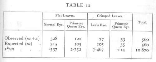
The expected values are calculated from the observed total, so that the four classes must agree in their sum, and if three classes are filled in arbitrarily the fourth is therefore determinate, hence n=3, [p. 82] χ²=10.87, the chance of exceeding which value is between .01 and .02; if we take P=.05 as the limit of significant deviation, we shall say that in this case the deviations from expectation are clearly significant.

Let us consider a second hypothesis in relation to the same data, differing from the first in that we suppose that the plants with crimped leaves are to some extent less viable than those with flat leaves. Such a hypothesis could of course be tested by means of additional data; we are only here concerned with the question whether or no it accords with the values before us. The hypothesis tells us nothing of what degree of relative viability to expect; we therefore take the totals of flat and crimped leaves observed, and divide each class in the ratio 3:1.

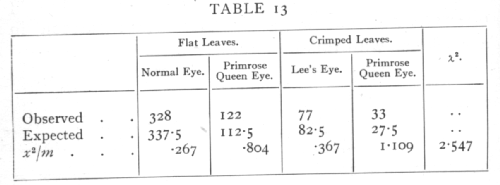
The value of n is now 2, since only two entries can be made arbitrarily; the value of χ², however, is so much reduced that P exceeds .2, and the departure from expectation is no longer significant. The significant part of the original discrepancy lay in the proportion of flat to crimped leaves.

It was formerly believed that in entering the χ² [p. 83] table n was always to be equated to one less than the number of frequency classes; this view led to many discrepancies, and has since been disproved with the establishment of the rule stated above. On the old view, any complication of the hypothesis such as that which in the above instance admitted differential viability, was bound to give us apparent improvement in the agreement between observation and hypothesis. When the change in n is allowed for this bias disappears, and if the value of P, rightly calculated; is many fold increased, as in this instance, the increase may safely be ascribed to an improvement in the hypothesis, and not to a mere increase of available constants.

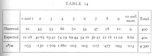
Ex. 9. Comparison with expectation of the Poisson Series and Binomial Series. -- In Table 5, p. 59, we give the observed and expected frequencies in the case of a Poisson Series. In applying the χ² test to such a series it is desirable that the number expected should in no group be less than 5, since the calculated distribution of χ² is not very closely realised for very small classes. We therefore pool the numbers for 0 and 1 cells, and also those for 10 and more, and obtain the following comparison:

[p.84]

Using 10 frequency classes we have χ²=4.390; in ascertaining the value of n we have to remember that the expected frequencies have been calculated, not only from the total number of values observed (400), but also from the observed mean; there remain, therefore, 8 degrees of freedom and n=8. For this value the χ² table shows that P is between .8 and .9, showing a close but not an unreasonably close, agreement with expectation.

Similarly in Table 10, p. 67, we have given the value of χ² based upon 12 classes for the two hypotheses of "true dice" and "biassed dice"; with "true dice" the expected values are calculated from the total number of observations alone, and n=11, but in allowing for bias we have brought also the means into agreement so that n is reduced to 10. In the first case χ² is far outside the range of the table showing a highly significant departure from expectation; in the second it appears that P lies between .2 and .3, so that the value of χ² is within the expected range.

A special and important class of cases where the agreement between expectation and observation may be tested comprises the tests of independence. If the same group of individuals is classified in two (or more) different ways, as persons may be classified as inoculated and not inoculated, and also as attacked and not attacked by a disease, then we may require to know if the two classifications are independent. [p. 85]

Ex. 10: Test of independence in a 2x2 classification. -- In the simplest case, when each classification comprises only two classes, we have a fourfold table, as in the following example (from Greenwood and Yule's data) for Typhoid:

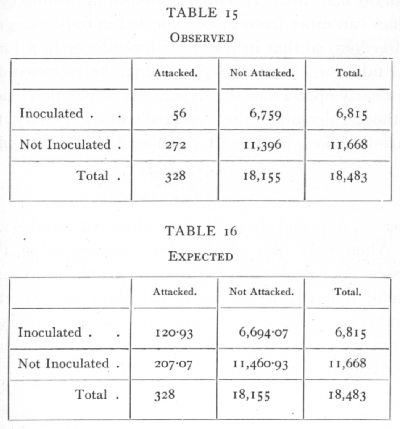
In testing independence we must compare the observed values with values calculated so that the four frequencies are in proportion; since we wish to test independence only, and not any hypothesis as to the total numbers attacked, or inoculated, the "expected" values are calculated from the marginal totals observed, so that the numbers expected agree with the numbers [p. 86] observed in the margins; only one value need be calculated, e.g.

the others are written down at once by subtraction from the margins. It is thus obvious that the observed values can differ from those expected in only 1 degree of freedom, so that in testing independence in a four; fold table, n =1. Since χ²=56.234 the observations are clearly opposed to the hypothesis of independence. Without calculating the expected values, χ² may, for fourfold tables, be directly calculated by the formula

where a, b, c, and d are the four observed numbers.

When only one of the classifications is of two classes, the calculation of χ² may be simplified to some extent, if it is not desired to calculate the expected numbers. If a, a' represent any pair of observed frequencies, and n, n' the corresponding totals, we calculate from each pair

and the sum of these quantities divided by nn' will be χ².

Ex. 11. Test of independence in a 2xn classification. -- From the pigmentation survey of Scottish children (Tocher's data) the following are the numbers of boys and girls from the same district (No. 1) whose hair colour falls into each of five classes: [p. 87]

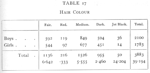
The quantities calculated from each pair of observations are given below in millions. Thus

approximately; the total of 39 millions odd divided by 2100 and by 1783 gives χ²=10.468· In this table 4 values could be filled in arbitrarily without conflicting with the marginal totals, so that n=4. The value of P is between .02 and .05, so that sex difference in the classification by hair colours is probably significant as judged by this district alone. The calculation of χ² from "expected" values, though somewhat more laborious, would have in this case the advantage of showing in which classes the boys, and in which classes the girls, were in excess. It appears from the numbers in the lowest line that the principle discrepancy is in the "Jet Black" class.

Ex. 12. Test of independence in a 4 x4 classification. -- As an example of a more complex contingency table we may take the results of a series of back-crosses [p. 88] in mice, involving the two Brown, Self-Piebald (Wachter's data):

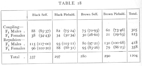
The back-crosses were made in four ways, according as the male or female parents were heterozygous (F₁) in the two factors, and according to whether the two dominant genes were received both from one (Coupling) or one from each parent (Repulsion).

The simple Mendelian ratios may be disturbed by differential viability, by linkage, or by linked lethals. Linkage is not suspected in these data, and if the only disturbance were due to differential viability the four classes in each experiment should appear in the same ratio; to test if the data show significant departures we may apply the χ² test to the whole 4x4 table. The values expected on the hypothesis that the proportions are independent of the matings used, or that the four series are homogeneous, are given above in brackets. The contributions to χ² made by each cell are given on page 89.

The value of χ² is therefore 21.832; the value of n is 9, for we could fill up a block of three rows and [p. 89]

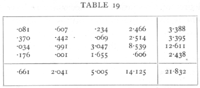
three columns and still adjust the remaining entries to check with the margins. In general for a contingency table of r rows and c columns n=(r-1)(c-1). For n=9, the value of χ² shows that P is less than .01, and therefore the departures from proportionality are not fortuitous; it is apparent that the discrepancy is due to the exceptional number of Brown Piebalds in the F₁ males repulsion series.

It should be noted that the methods employed in this chapter are not designed to measure the degree of association between one classification and another, but solely to test whether the observed departures from independence are or are not of a magnitude ascribable to chance. The same degree of variation may be significant for a large sample but insignificant for a small one; if it is insignificant we have no reason on the data present to suspect any degree of association at all, and it is useless to attempt to measure it. If, on the other hand, it is significant the value of χ² indicates the fact, but does not measure the degree of association. Provided the deviation is clearly significant, it is of no practical importance whether P is .01 or ·.000,001, and it is for this reason that we have not tabulated the value of χ² beyond .01. To measure [p. 90] the degree of association it is necessary to have some hypothesis as to the nature of the departure from independence to be measured. With Mendelian frequencies, for example, the cross-over percentage may be used to measure the degree of association of two factors, and the significance of evidence for linkage may be tested by comparing the difference between the cross-over percentage and 50 per cent (the value for unlinked factors), with its standard error. Such a comparison, if accurately carried out, must agree absolutely with the conclusion drawn from the χ² test. To take a second example, the values in a four-fold table may be sometimes regarded as due to the partition of a normally correlated pair of variates, according as the values are above or below arbitrarily chosen dividing-lines ; as if a group of stature measurements of fathers and sons were divided between those above and those below 68 inches. In this case the departure from independence may be properly measured by the correlation in stature between father and son; this quantity can be estimated from the observed frequencies, and a comparison between the value obtained and its standard error, if accurately carried out, will agree with the χ² test as to the significance of the association; the significance will become more and more pronounced as the sample is increased in size, but the correlation obtained will tend to a fixed value. The χ² test does not attempt to measure the degree of association, but as a test of significance it is independent of all additional hypotheses as to the nature of the association. [p. 91]

Tests of homogeneity are mathematically identical with tests of independence; the last example may equally be regarded in either light. In Chapter III. the tests of agreement with the Binomial Series were essentially tests of homogeneity; the ten samples of 100 ears of barley (Ex. 7, p. 72) might have been represented as a 2x10 table. The χ² index of dispersion would then be equivalent to the χ² obtained from the contingency table. The method of this chapter is more general, and is applicable to cases in which the successive samples are not all of the same size.

Ex. 13· Homogeneity of different families in respect of ratio black: red. -- The following data show in 33 families of Gammarus (Huxley's data) the numbers with black and red eyes respectively:

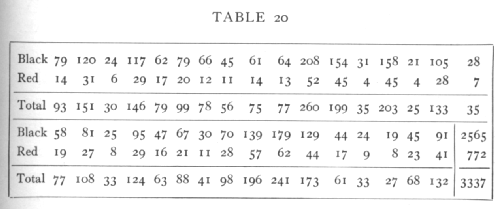
The totals 2565 black and 772 red are distinctly not in the ratio 3:1, which is ascribed to linkage. The question before us is whether or not all the families indicate the same ratio between black and red, or whether the discrepancy is due to a few families only. For the whole table χ²=35.620, n=32. This is [p. 92] beyond the range of the table, so we apply the method explained on p. 63:

The series is therefore not significantly heterogeneous; effectively all the families agree and confirm each other in indicating the black-red ratio observed in the total.

Exactly the same procedure would be adopted if the black and red numbers represented two samples distributed according to some character or characters each into 33 classes. The question "Are these samples of the same population?" is in effect identical with the question "Is the proportion of black to red the same in each family?" To recognise this identity is important, since it has been very widely disregarded.

Ex. 14· Agreement with expectation of normal variance. -- Closely akin to tests of homogeneity is the use of the χ² distribution to test whether or not an observed series of values, normally or nearly normally distributed, agrees in its variance with expectation. If x₁, x₂,..., are a sample of a normal population, the standard deviation of which population is s, then

is distributed in random samples as is χ², taking n one less than the number of the sample. J. W. Bispham gives three series of experimental values of the partial correlation coefficient, which he assumes should be [p. 93] distributed so that 1/s²=29, but which theoretically should have 1/s²=28. Th, values of S(x-x[bar])² for the three samples of 1000, 200, 100 respectively are, as judged from the grouped data,

35.0278, 7.1071, 3.6169,

whence the values of χ² on the two theories are

It will be seen that the true formula for the variance gives slightly the better agreement. That the difference is not significant may be seen from the last two columns. About 6000 observations would be needed to discriminate experimentally, with any certainty, between the two formulæ.

Just as values of χ² may be aggregated together to make a more comprehensive test, so in some cases it is possible to separate the contributions to χ² made by the individual degrees of freedom, and so to test the separate components of a discrepancy.

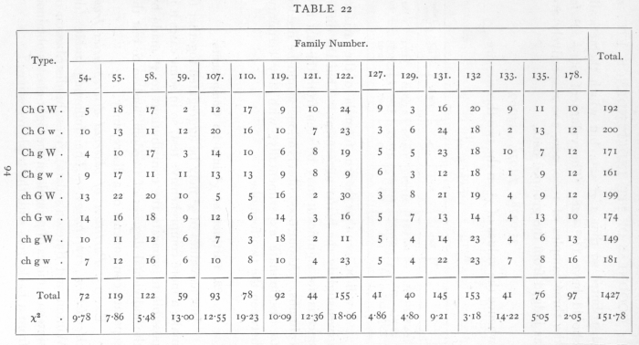
Ex. I5· Partition of observed discrepancies from Mendelian expectation. -- The following table (de Winton and Bateson's data) gives the distribution of sixteen families of primula in the eight classes obtained from a back-cross with the triple recessive: [p. 94]

 [p. 95]

The theoretical expectation is that the eight classes should appear in equal numbers, corresponding to the hypothesis that in each factor the allelomorphs occur with equal frequency, and that the three factors are unlinked. This expectation is fairly realised in the totals of the sixteen families, but the individual families are somewhat irregular. The values of χ² obtained by comparing each family with expectation are given in the lowest line. These values each correspond to seven degrees of freedom, and it appears that in 5 cases out of 16, P is less than .1, and of these 2 are less than .02. This confirms the impression of irregularity, and the total value of χ² (not to be confused with χ² derived from the totals), which corresponds to 112 degrees of freedom, is 151.78. Now

so that, judged by the total χ², the evidence for departures from expectation in individual families, is clear.

Each family is free to differ from expectation in seven independent ways. To carry the analysis further, we must separate the contribution to χ² of each of these seven degrees of freedom. Mathematically the subdivision may be carried out in more than one way, but the only way which appears to be of biological interest is that which separates the parts due to inequality of the allelomorphs of the three factors, and the three possible linkage connexions. If we separate [p. 95] the frequencies into positive and negative values according to the following seven ways,

then it will be seen that all seven subdivisions are wholly independent, since any two of them agree in four signs and disagree in four. The first three degrees of freedom represent the inequalities in the allelomorphs of the three factors Ch, G, and W; the next are the degrees of freedom involved in an enquiry into the linkage of the three pairs of factors, while the seventh degree of freedom has no simple biological meaning but is necessary to complete the analysis. If we take in the first family, for example, the difference between the numbers of the W and w plants, namely 8, then the contribution of this degree of freedom to χ² is found by squaring the difference and dividing by the number in the family, e.g. 82/72=889. In this way the contribution of each of the 112 degrees of freedom in the sixteen families is found separately, as shown in the following table: [p. 97]

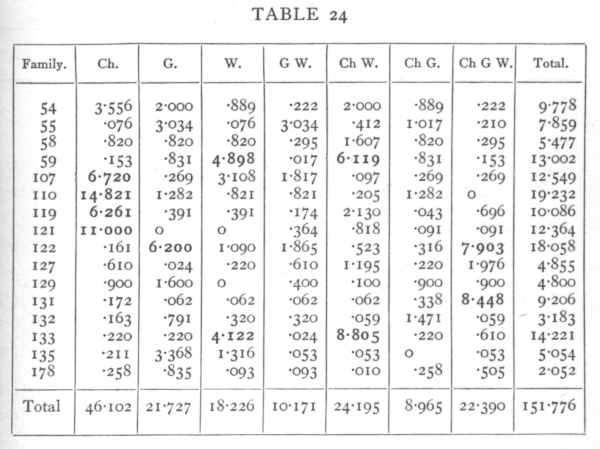
Looking at the total values of χ² for each column, since n is 16 for these, we see that all except the first have values of P between .05 and .95, while the contribution of the first degree of freedom is very clearly significant. It appears then that the greater part, if not the whole, of the discrepancy is ascribable to the behaviour of the Sinensis-Stellata factor, and its behaviour strongly suggests close linkage with a recessive lethal gene of one of the familiar types. In four families, 107-121, the only high contribution is in the first column. If these four families are excluded χ²=97.545, and this exceeds the expectation for n=84 by only just over the standard error; the total discrepancy cannot therefore be regarded as significant. There does, however, appear to be an excess of very large entries, and it is noticeable of the seven largest, [p. 98-99]

 [p. 100]

six appear in pairs belonging to the same family. The distribution of the remaining 12 families according to the value of P is as follows:

from which it would appear that there is some slight evidence of an excess of families with high values of χ². This effect, like other non-significant effects, is only worth further discussion in connexion with some plausible hypothesis capable of explaining it.

N.B. -- Table of χ², p. 98.